Spatial Aggregation & Areal Interpolation

Today

1. The problem — data in the wrong zones
2. Support — what does a value attached to a polygon mean?
3. Extensive vs. intensive — what happens when you split a geometry?
4. Areal interpolation in R — st_interpolate_aw() and st_agr()
5. Limitations — when the uniform assumption fails; dasymetric mapping

The Problem

Data in the wrong zones

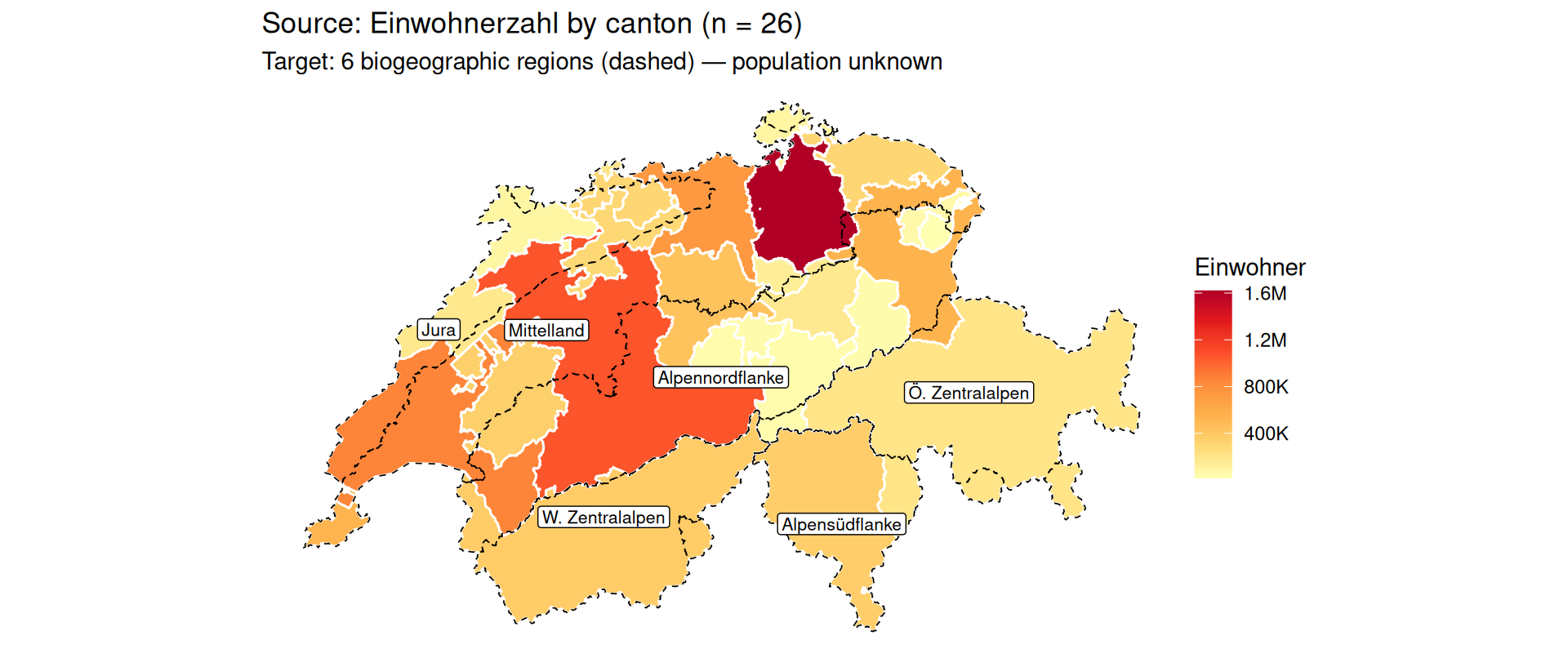
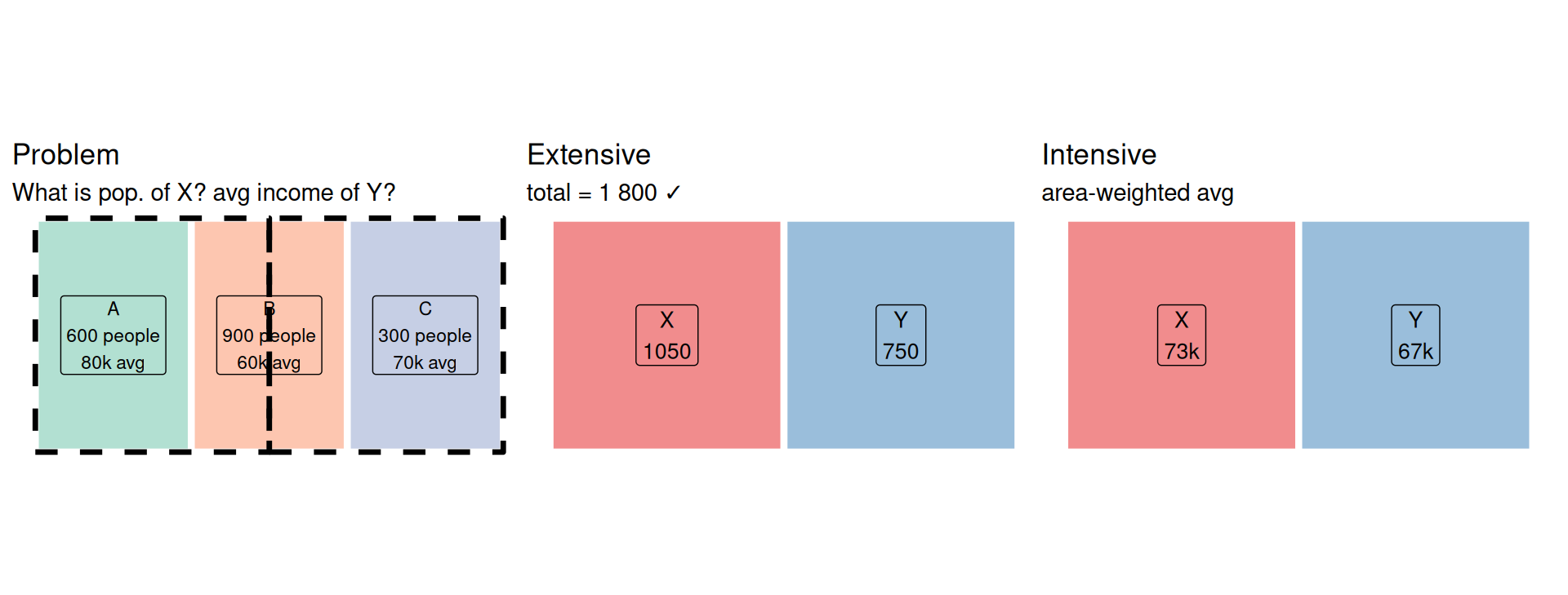
You have data — but the zones don’t match what you need:

• Population by canton, but you need it by biogeographical region
• Income by census tract, but you need it by school district

The source zones and target zones overlap in arbitrary ways. You cannot simply reassign values — you have to redistribute them.

Areal interpolation is the second largest source of error in spatial data science.

Edzer Pebesma - Areal interpolation methods - useR! 2026

Students often assume this is a rare edge case. It is not. Any time you combine data from different administrative sources — census, tax, health, transport — you face this problem. The error compounds silently: results look reasonable but are systematically wrong.

The core challenge

Walk through the problem: target zone X overlaps with all of A and half of B. You cannot just assign A’s population to X — X also covers part of B. You need to split B’s population between X and Y based on how much of B falls in each target zone.

Support

Q1: What does the value refer to?

Before you can redistribute a variable, you need to know what it represents.

• Point support — the value refers to each individual location: E.g. Land cover, soil type
• Block support — the value refers to the whole geometry as a unit: E.g. Population count, average income

Point-support variables can be sampled and re-aggregated without conceptual difficulty. Block-support variables cannot — they are aggregates, and their spatial distribution within the polygon is unknown. Areal interpolation only applies to block-support variables.

Why support matters

• For point-support variables: you can query any sub-region directly. A raster crop, a spatial filter, a point-in-polygon lookup — all valid.
• For block-support variables: the value only makes sense for the whole geometry. Splitting it requires an assumption about how the variable is distributed within the polygon.
  • The simplest assumption: uniform distribution — the variable is spread evenly across the area.
  • This assumption is almost never true

Extensive vs. Intensive

For Block support

Q2: What happens when you cut a polygon in half?

Question: does the value sum across sub-regions, or does it stay constant?

Variable	Cut in half →	Type
Population count (1 000)	~500 each	Extensive
Population density (50/km²)	still 50/km² each	Intensive
Total household income (€200M)	~€100M each	Extensive
Average household income (€60k)	still €60k each	Intensive
Number of schools (12)	~6 each	Extensive
School density (2/km²)	still 2/km²	Intensive

Extensive = summable = total. Intensive = per-unit = rate or density or average. The confusion between the two is a classic error in spatial analysis — e.g. summing population densities instead of averaging them, or averaging population counts instead of summing them.

Redistribution formulas

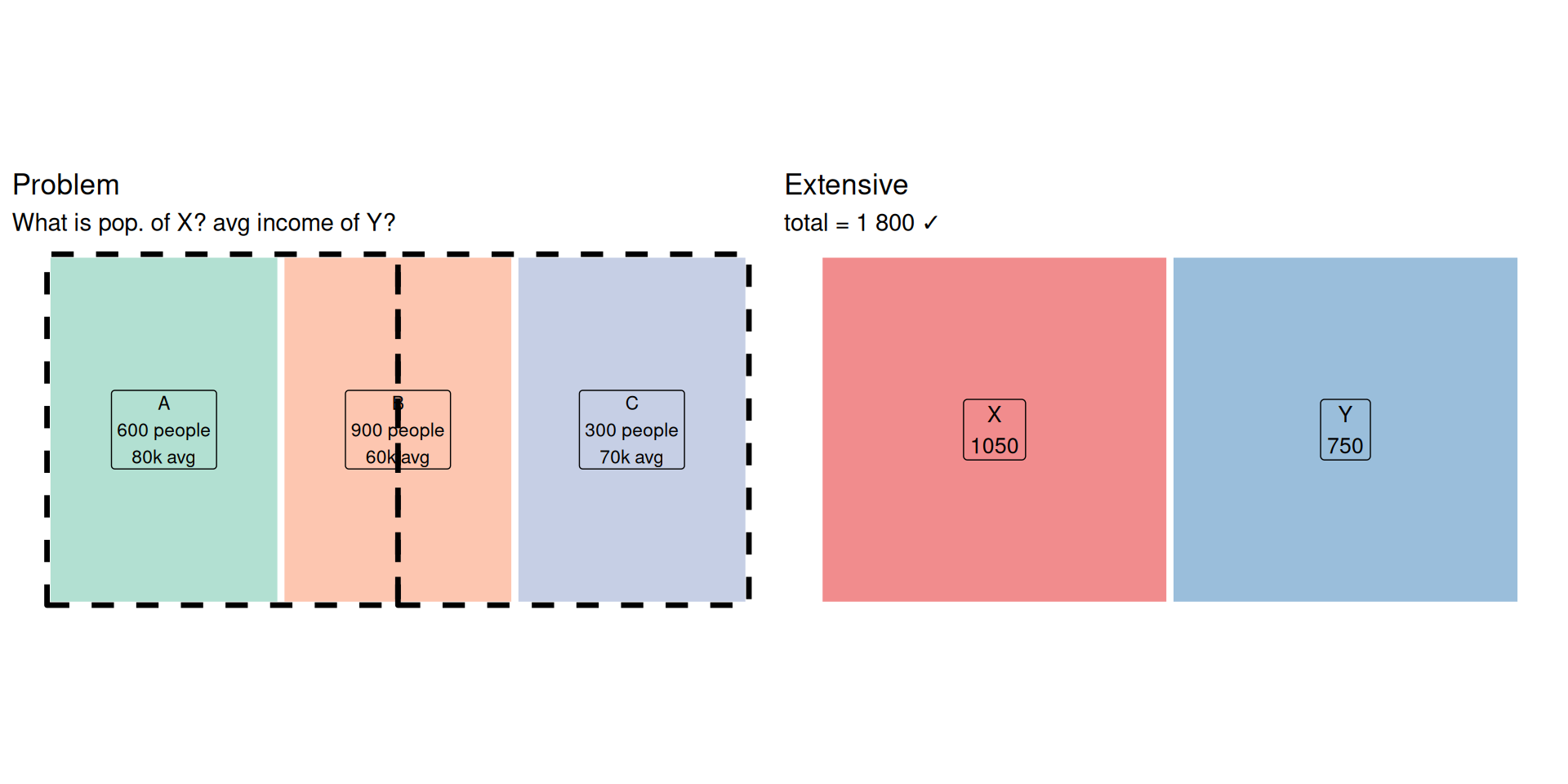
Extensive (counts, totals — the sum must be preserved):

\[v_j = \sum_i v_i \cdot \frac{\text{area}(A_i \cap B_j)}{\text{area}(A_i)}\]

Each source value is split proportionally to the area of intersection.

Intensive (rates, densities, averages — no sum to preserve):

\[v_j = \frac{\displaystyle\sum_i v_i \cdot \text{area}(A_i \cap B_j)}{\displaystyle\sum_i \text{area}(A_i \cap B_j)}\]

Each source value is weighted by the intersection area, then averaged.

How to read the formulas — use the toy example (A/B/C → X/Y):

• \(i\) indexes source zones (A, B, C); \(j\) indexes target zones (X, Y)
• \(v_i\) is the value in source zone \(i\) (e.g. 900 people in B)
• \(A_i \cap B_j\) is the intersection of source zone \(i\) with target zone \(j\) (e.g. the left half of B that falls in X)
• \(\text{area}(A_i \cap B_j) / \text{area}(A_i)\) is the area fraction — what share of source zone \(i\) overlaps target zone \(j\). B∩X = 50%, so 0.5 × 900 = 450.

Extensive: sum contributions from all source zones touching \(j\), each scaled by area fraction. For X: 100%×600 + 50%×900 = 1 050.

Intensive: area-weighted average — weight each source value by how much of the target it covers. For Y: B covers 1 unit, C covers 2 units → (60×1 + 70×2)/3 = 66.7 k.

Key contrast: extensive preserves the total (1 800 in, 1 800 out). Intensive preserves the scale of the variable (still CHF/year, not CHF·km²/year).

Areal Interpolation in R

st_interpolate_aw()

# extensive = TRUE  →  sum-preserving (counts, totals)
pop_by_target <- st_interpolate_aw(src["population"], tgt, extensive = TRUE)

Warning in st_interpolate_aw.sf(src["population"], tgt, extensive = TRUE):
st_interpolate_aw assumes attributes are constant or uniform over areas of x

• Notice the warning: assumes attributes are constant or uniform over areas of x
• This is the uniform distribution assumption — built into the method.

Declaring attribute support: st_agr()

st_agr(src)                          # NA = undeclared

      zone population income_avg 
      <NA>       <NA>       <NA> 
Levels: constant aggregate identity

st_agr(src) <- c(population = "aggregate",   # block, summable  → extensive = TRUE
                 income_avg = "constant")     # spatially constant → extensive = FALSE
st_agr(src)

      <NA> population income_avg 
      <NA>  aggregate   constant 
Levels: constant aggregate identity

• "aggregate" — block support, summable total: use extensive = TRUE
• "constant" — spatially constant or rate: use extensive = FALSE

Setting this suppresses the warning and lets sf propagate attribute semantics correctly through operations like st_intersection().

# extensive = FALSE  →  area-weighted average (rates, densities)
inc_by_target <- st_interpolate_aw(src["income_avg"], tgt, extensive = FALSE)
inc_by_target$zone <- c("X", "Y")
inc_by_target$income_avg

[1] 73.33333 66.66667

The function is honest: it warns you that it’s making an assumption you may not have thought about. Many students suppress warnings. This is a case where the warning is the most important part of the output.

Population totals: A=600, B=900, C=300. X covers all of A (600) plus half of B (450) = 1050. Y covers half of B (450) plus all of C (300) = 750. Sum = 1800. Preserved ✓

Income averages: X covers A (80, weight 2) and half of B (60, weight 1) → (160+60)/3 = 73.3. Y covers half of B (60, weight 1) and C (70, weight 2) → (60+140)/3 = 66.7.

Limitations

When the uniform assumption fails

The uniform distribution assumption is wrong whenever the variable is spatially heterogeneous within the source zone.

Examples:

• Population in a municipality that is 80% forest → people cluster in villages, not forest
• Income data for a large canton → urban and rural areas have very different incomes
• Large source zones intersecting many small target zones → fine-grained heterogeneity is lost

Dasymetric mapping

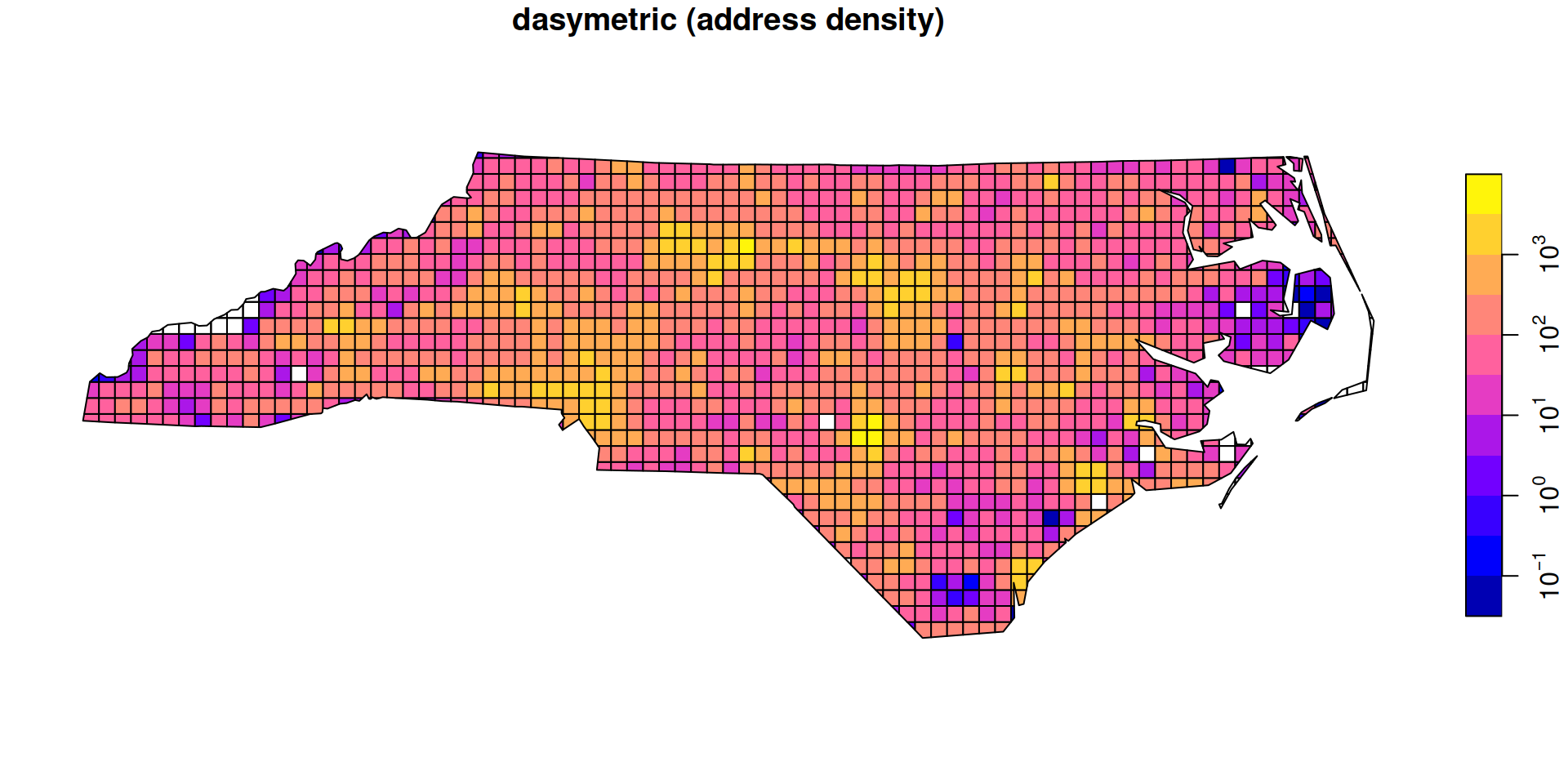
• Improve accuracy by using ancillary data that captures spatial heterogeneity within the source zone.
• Classic example — population redistribution:
  1. Overlay source zones with land use / building footprint data
  2. Assign population only to residential areas
  3. Intersect with target zones and sum
• The more precise the ancillary layer, the more accurate the result.
• In R: pass the ancillary layer as weights = to st_interpolate_aw().
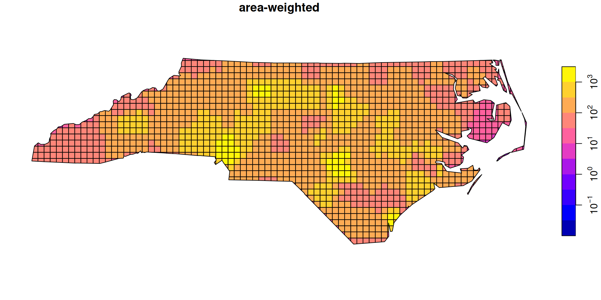
• Example from r-spatial.github.io/sf

Dasymetric mapping is the standard improvement over naive areal weighting. It’s especially important when source zones are large relative to the variation in the variable. The key limitation: you need a good ancillary layer, which itself may be outdated or imprecise.

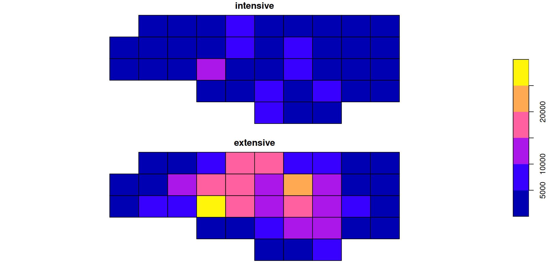
Intensive vs extensive — side by side

nc <- st_read(system.file("shape/nc.shp", package = "sf"), quiet = TRUE)
g  <- st_make_grid(nc, n = c(10, 5))

a1 <- st_interpolate_aw(nc["BIR74"], to = g, extensive = FALSE)
a2 <- st_interpolate_aw(nc["BIR74"], to = g, extensive = TRUE)
sum(a2$BIR74) / sum(nc$BIR74)   # mass preserved → 1

[1] 0.9999998

Intensive and extensive give visually different results even on the same data. The extensive result preserves the total count (ratio → 1). The intensive result does not — it spreads values as if they were uniform rates, so the sum drifts. This is the core reason the distinction matters.

Dasymetric mapping in R

grd.addr <- read_sf(system.file("gpkg/grd_addr.gpkg", package = "sf"))
nc2 <- st_transform(nc, st_crs(grd.addr))
st_agr(grd.addr) <- c(ones = "constant")
st_agr(nc2)      <- c(BIR74 = "constant")

bir0 <- st_interpolate_aw(nc2["BIR74"], to = grd.addr, extensive = TRUE)
bir1 <- st_interpolate_aw(nc2["BIR74"], to = grd.addr, extensive = TRUE,
                           weights = "ones")
sum(bir1$BIR74) / sum(nc2$BIR74)   # mass preserved → 1

[1] 1

grd.addr contains ones = number of postal addresses per 10 km grid cell — a proxy for where people actually live. weights = "ones" tells st_interpolate_aw() to weight intersections by this ancillary variable instead of by raw area. The dasymetric result concentrates births in populated cells.

Mass preservation: sum(bir1$BIR74) / sum(nc2$BIR74) → 1. The pycnophylactic property holds regardless of the ancillary layer.

Roundtrip verification: interpolate the grid back to county boundaries and compare with the original — the scatter plot should hug the 1:1 line.