Spherical Geometry in sf

Today

1. S² and R² — two models of space, one hidden default
2. When flat breaks — antimeridian rendering and predicate failures
3. A polygon has two sides — the core challenge of spherical geometry
4. Semi-open boundaries — why adjacent polygons share more than a border
5. Discussion — when does it matter in practice?

S² and R²

Two models of space

R² (flat)

• Points are (x, y) on an infinite plane
• Used by GEOS — the geometry engine behind QGIS, PostGIS, sf historically
• Assumes straight lines, Euclidean distances
• Appropriate for projected CRS

S² (sphere)

• Points are (lon, lat) on a unit sphere
• Used by s2 — Google’s C++ spherical geometry library, wrapped by the s2 R package
• Lines follow great circles; distances are geodesic
• Appropriate for geographic CRS
• Powers Google Maps, Earth Engine, and BigQuery GIS

The switch

• Since sf version 1.0 (2021), geographic coordinates automatically use s2 instead of GEOS.
• Same function call; different geometry engine; potentially very different results
• The switch affects: st_area(), st_length(), st_distance(), st_buffer(), all predicates

sf_use_s2()        # check current engine

[1] TRUE

sf_use_s2(FALSE)   # switch to GEOS (flat, R²)
sf_use_s2(TRUE)    # switch back to s2 (spherical, S²)

This is the key lever. When students see unexpected results with geographic data, checking sf_use_s2() is a good first step. Most of the time s2 gives the right answer; occasionally an operation isn’t yet implemented and you need to fall back to GEOS.

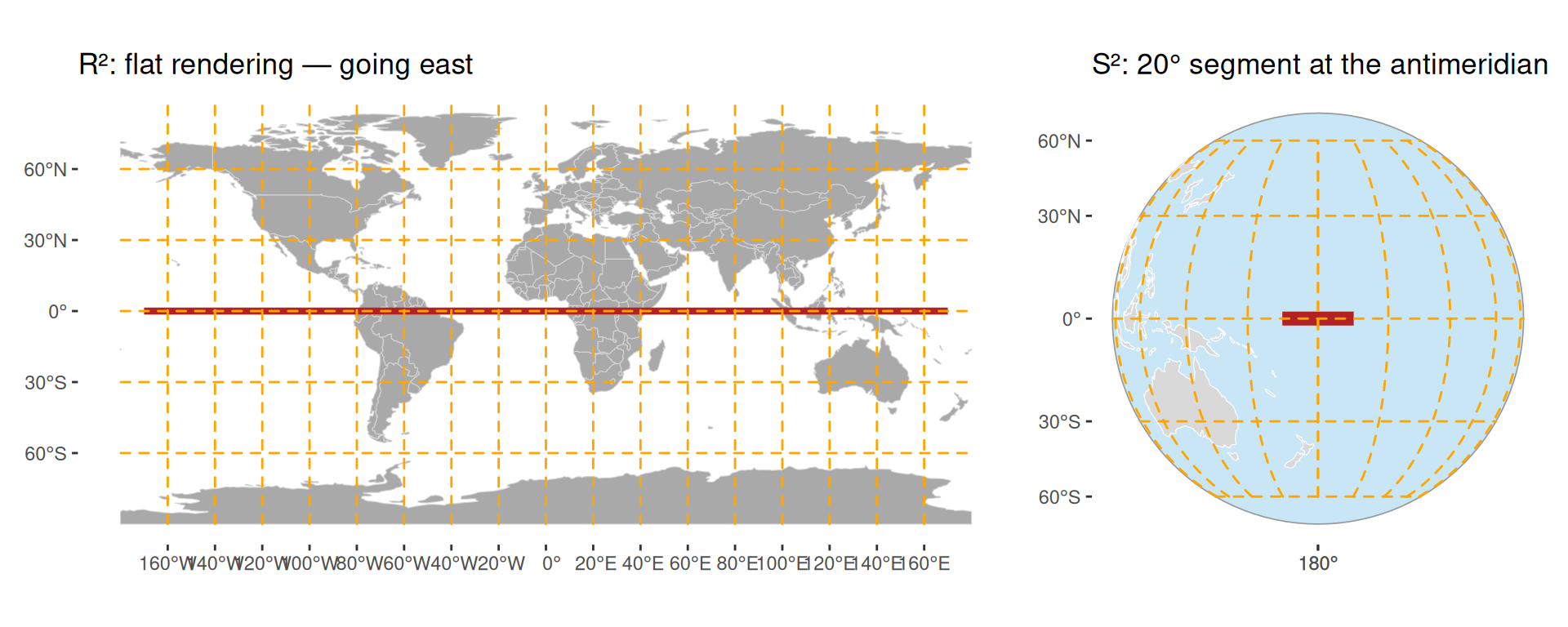
When flat breaks: the antimeridian

Same two endpoints — completely different rendering:

In R² the line is drawn as a straight horizontal segment from -170 to +170 going EAST across the globe — 340° of longitude on the flat map. In S², the same two points are connected by the short great-circle arc going WEST across the antimeridian — just 20°. Same two coordinates, completely different rendering. Note: st_length gives essentially the same result under both engines because GEOS also computes the minimum geodesic distance for a 2-point line; the difference shows up in how the geometry is drawn and in spatial operations on more complex shapes.

When flat breaks: predicates

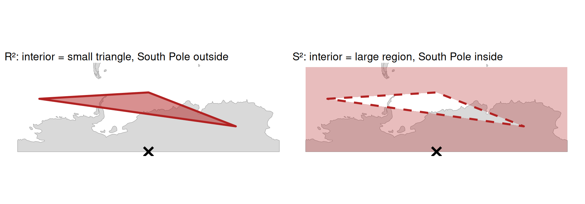
The same polygon, the same point — different answer:

sf_use_s2(FALSE)
st_contains(pol, pole)   # R²: pole is outside

Sparse geometry binary predicate list of length 1, where the predicate
was `contains'
 1: (empty)

sf_use_s2(TRUE)
st_contains(pol, pole)   # S²: pole is inside

Sparse geometry binary predicate list of length 1, where the predicate
was `contains'
 1: 1

In R², the polygon edges are straight lines in equirectangular space. The three vertices form a small triangle that sits above the South Pole — the pole is clearly outside. In S², the edges follow great circles. Great-circle arcs between points in the southern hemisphere curve toward the pole, so the same three vertices enclose a much larger region that includes the South Pole. Same coordinates, opposite predicate result. Source: Pebesma & Dunnington (2020), “In r-spatial, the Earth is no longer flat”.

A polygon has two sides

Two regions from one ring

In R²: a polygon ring encloses a bounded area. The outside extends to infinity — obviously “outside.”

In S²: a ring on a sphere divides it into exactly two finite regions. There is no infinity. Which side is “inside” depends entirely on ring direction.

# Same 4 corners — different winding order
sq_ccw <- st_sfc(st_polygon(list(matrix(          # CCW → small region
  c(-10,-10, 10,-10, 10,10, -10,10, -10,-10),
  ncol = 2, byrow = TRUE))), crs = 4326)

sq_cw  <- st_sfc(st_polygon(list(matrix(          # CW  → large region
  c(-10,-10, -10,10, 10,10, 10,-10, -10,-10),
  ncol = 2, byrow = TRUE))), crs = 4326)

units::set_units(st_area(sq_ccw), "km^2")   # small square

4969697 [km^2]

units::set_units(st_area(sq_cw),  "km^2")   # rest of Earth

4969697 [km^2]

Ring direction

• In S²: interior is the region to the left when walking the boundary
• CCW ring (counter-clockwise) → interior is the small side — same as R²
• CW ring (clockwise) → interior is the large side — the “rest of the globe”

Ring	R² behaviour	S² behaviour
CCW exterior	Standard polygon	Small-side interior
CW exterior	Invalid / hole	Large-side interior

• st_as_s2(x, oriented = FALSE) auto-corrects ring direction, assuming the intended interior is less than half the sphere

Stop and think

You are building a global land cover database. One of the classes is ocean.

How would you represent the ocean as a geometry in a GIS?

Discuss in pairs. Consider:

• What are its boundaries?
• Can you define it as a simple polygon in R²?
• What about in S²?

The ocean is the complement of all land polygons — it has no outer boundary, only inner ones.

In R²: impossible to represent directly (unbounded exterior).

In S²: the whole sphere is a valid polygon.

land  <- st_as_sf(s2_data_countries())
earth <- st_as_sfc("POLYGON FULL", crs = "EPSG:4326")
ocean <- st_difference(earth, st_union(land))

# Fraction of Earth's surface covered by ocean
as.numeric(st_area(ocean) / st_area(earth))

[1] 0.288699

Semi-open boundaries

The shared edge problem

Adjacent polygons share an edge. Under S² (or GEOS with model = "closed"):

• A point on the shared edge intersects both polygons
• For spatial joins or point-in-polygon counts: double-counting

# Default: closed model — adjacent counties intersect each other
st_intersects(nc[1:3, ], nc[1:3, ], sparse = FALSE)

      [,1] [,2]  [,3]
[1,]  TRUE TRUE FALSE
[2,]  TRUE TRUE  TRUE
[3,] FALSE TRUE  TRUE

# Semi-open: each county only intersects itself
st_intersects(nc[1:3, ], nc[1:3, ], sparse = FALSE, model = "semi-open")

      [,1]  [,2]  [,3]
[1,]  TRUE FALSE FALSE
[2,] FALSE  TRUE FALSE
[3,] FALSE FALSE  TRUE

The model parameter controls boundary inclusion:

Model	Boundary belongs to	Use when
"closed" (default)	Both polygons	Spatial filters, overlap detection
"open"	Neither polygon	Points strictly inside only
"semi-open"	Exactly one polygon	Coverage operations, point-in-polygon counts, raster analogy

The semi-open model mirrors how raster grids work: each cell owns its upper-left corner and upper/left edges — no gaps, no double-counting.

Practical consequences

How different are measurements?

For typical geographic analyses: negligible.

Measure	Relative difference (s2 vs flat)	Absolute example
Area	±0.007%	~7 km² per 100 000 km²
Length	±0.013%	~13 m per 100 km
Distance	up to ~0.5%	~1–2 km over 500 km

For continental or global scale: not negligible. The antimeridian is the clearest failure case.

When to use each engine

sf_use_s2(TRUE)   # default — always correct for geographic CRS
sf_use_s2(FALSE)  # fall back to GEOS when:
                  #  • working with projected CRS (s2 adds no benefit)
                  #  • an operation is not yet in s2 (e.g. st_voronoi())
                  #  • debugging: compare results between engines

Rule of thumb:

• Geographic CRS (degrees) → leave s2 on
• Projected CRS (metres) → irrelevant which engine; GEOS is used anyway
• Operation fails or warns → check if the operation is implemented in s2; fall back if needed

Discussion

Discussion challenge

Your colleague downloads Swiss municipality boundaries in EPSG:4326 and runs:

municipalities |>
  st_join(cantons, join = st_intersects) |>
  group_by(canton_id) |>
  summarise(total_pop = sum(pop))

Some municipalities on cantonal borders appear in two cantons and their population is counted twice.

• What is causing this?
• How do you fix it?
• Are there cases where model = "closed" is actually the right choice?

Discuss in groups

No external sources — reason from what you know about s2 boundary models

References