Original: 828324 vertices100 m tolerance: 40056 vertices1 000 m tolerance: 27885 vertices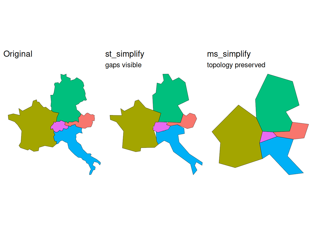
Practice the geometry operations from today’s lecture using Swiss spatial data.
These tasks were specifically designed to be solvable without AI. Solve them without it!
Compare how st_simplify() and ms_simplify() behave, and discover the topology problem.
Data (available on Moodle, under Spatial Analysis II):
swissBOUNDARIES3D.gpkg — Canton of Luzern boundary
swiss_TLM3D.gpkg, layer tlm_bb — land cover polygons with attribute objektart
1.1 Load forest polygons (objektart == "Wald") within Canton Luzern. Apply st_simplify() with tolerances of 100 m and 1 000 m. How many vertices does each version have compared to the original?
1.2 Load Switzerland and its four neighbours (Germany, France, Austria, Italy) using rnaturalearth::ne_countries(), transform to EPSG:3857. Apply st_simplify() with a tolerance of 50 000 m. Do gaps appear between countries?
1.3 Apply rmapshaper::ms_simplify() with keep = 0.1 to the same dataset. How do the shared borders compare?
1.4 Map all three versions side by side.
Original: 828324 vertices100 m tolerance: 40056 vertices1 000 m tolerance: 27885 vertices
Switzerland reports economic output (GDP) by canton. But canton boundaries don’t match ecological or planning zones. How much of Switzerland’s GDP comes from the Alps vs. the Mittelland?
In this exercise you will redistribute cantonal GDP to Switzerland’s 6 biogeographic regions using areal interpolation.
Data (all in this project’s data/ folder):
swissboundaries-cantons.gpkg — 26 cantons with name and einwohnerzahlgdp-canton-CH.csv — cantonal GDP 2011–2024 in CHF million (BFS, retrieved 2026-11-09)biogeo.gpkg — 6 biogeographic regions with RegionNummer and region_de2.1 Load the canton geometries (layer tlm_kantonsgebiet).
2.2 Read gdp-canton-CH.csv. Select only name and gdp_2024, then join to the canton geometries. Verify: are there any unmatched cantons?
2.3 Which three cantons have the highest total GDP (gdp_2024)? Does the result surprise you?
2.4 Is gdp_2024 an extensive or intensive variable? Declare it with st_agr().
2.5 Load data/biogeo.gpkg. Inspect the result: how many features, which columns?
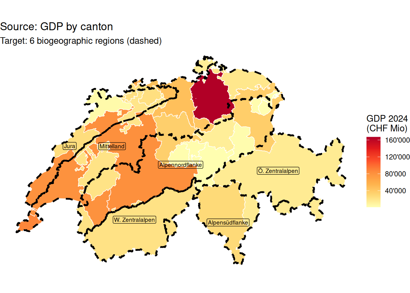
2.6 Map cantons (fill by gdp_2024) with biogeographic region boundaries overlaid as a dashed outline.
2.7 Redistribute total GDP to biogeographic regions (extensive = TRUE). Verify mass is preserved: sum(result$gdp_2024) / sum(cantons$gdp_2024) should equal 1. Which region has the highest total GDP?
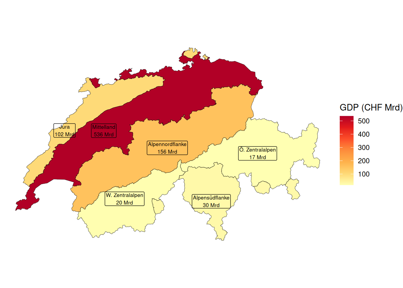
2.8 Map the result.